Docking#
This tutorial showcases how to use ProLIF to generate an interaction fingerprint for interactions between a protein and different docking poses.
ProLIF currently provides file readers for docking poses for MOL2, SDF and PDBQT files which rely on RDKit or MDAnalysis (or both).
Important
For convenience, the different files for this tutorial are included with the ProLIF installation, and we’ll access these files through plf.datafiles.datapath which is a pathlib.Path object pointing to the tutorials data directory. This makes it easier to manipulate paths to files, match filenames using wildcards…etc. in a Pythonic way, but you can also use plain strings, e.g. "/home/user/prolif/data/vina/rec.pdb" instead of plf.datafiles.datapath / "vina" / "rec.pdb" if you prefer.
Remember to replace any reference to plf.datafiles.datapath with the actual paths to your inputs outside of this tutorial.
Tip
At the top of the page you can find links to either download this notebook or run it in Google Colab. You can install the dependencies for the tutorials with the command:
pip install prolif[tutorials]
Protein preparation#
Let’s start by importing MDAnalysis and ProLIF to read our protein for this tutorial.
In this tutorial we’ll be using a PDB file but you can also use the MOL2 format as shown later on.
Important
No matter which file format you chose to use for the protein, it must contain explicit hydrogens.
PDB file#
We have 2 options to read the protein file: MDAnalysis (preferred) or RDKit (faster but risky, see below).
Important
While RDKit is going to be much faster at parsing the file, it can only recognize standard residue names, so some protonated residues may be incorrectly parsed.
For example, the protonated histidine residue HSE347 in our protein is not correcltly parsed which removes aromaticity on the ring, meaning that ProLIF will not be able to match this residue for pi-stacking interactions.
import prolif as plf
from rdkit import Chem

protein_file = str(plf.datafiles.datapath / "vina" / "rec.pdb")

rdkit_prot = Chem.MolFromPDBFile(protein_file, removeHs=False)
protein_mol = plf.Molecule(rdkit_prot)
# histidine HSE347 not recognized by RDKit
plf.display_residues(protein_mol, slice(260, 263))
/home/docs/checkouts/readthedocs.org/user_builds/prolif/envs/latest/lib/python3.11/site-packages/MDAnalysis/topology/TPRParser.py:161: DeprecationWarning: 'xdrlib' is deprecated and slated for removal in Python 3.13
  import xdrlib

Unless you know for sure that all the residue names in your PDB file are standard, it is thus recommanded that you use MDAnalysis for parsing the protein.
import MDAnalysis as mda
import prolif as plf

u = mda.Universe(protein_file)
protein_mol = plf.Molecule.from_mda(u)
# display (remove `slice(260, 263)` to show all residues)
plf.display_residues(protein_mol, slice(260, 263))

Important
Make sure that your PDB file either has all bonds explicitely stated, or none of them.
Troubleshooting
In some cases, some atomic clashes may be incorrectly classified as bonds and will prevent the conversion of the MDAnalysis molecule to RDKit through ProLIF. Since MDAnalysis uses van der Waals radii for bond detection, one can modify the default radii that are used:
u.atoms.guess_bonds(vdwradii={"H": 1.05, "O": 1.48})
MOL2 file#
You could also use a MOL2 file for the protein, here’s a code snippet to guide you:
u = mda.Universe("protein.mol2")
# add "elements" category
elements = mda.topology.guessers.guess_types(u.atoms.names)
u.add_TopologyAttr("elements", elements)
# create protein mol
protein_mol = plf.Molecule.from_mda(u)
Troubleshooting
While doing so, you may run into one of these errors:
RDKit ERROR: Can't kekulize mol. Unkekulized atomsRDKit ERROR: non-ring atom marked aromatic
This usually happens when some of the bonds in the MOL2 file are unconventional. For example in MOE, charged histidines are represented part with aromatic bonds and part with single and double bonds, presumably to capture the different charged resonance structures in a single one. A practical workaround for this is to redefine problematic bonds as single bonds in the Universe object:
u = mda.Universe("protein.mol2")
# replace aromatic bonds with single bonds
for i, bond_order in enumerate(u._topology.bonds.order):
    # you may need to replace double bonds ("2") as well
    if bond_order == "ar":
        u._topology.bonds.order[i] = 1
# clear the bond cache, just in case
u._topology.bonds._cache.pop("bd", None)
# infer bond orders again
protein_mol = plf.Molecule.from_mda(u)
The parsing of residue info in MOL2 files can sometimes fail and lead to the residue index being appended to the residue name and number. You can fix this with the following snippet:
import numpy as np

u = mda.Universe("protein.mol2")
resids = [
    plf.ResidueId.from_string(x) for x in u.residues.resnames
]
u.residues.resnames = np.array([x.name for x in resids], dtype=object)
u.residues.resids = np.array([x.number for x in resids], dtype=np.uint32)
u.residues.resnums = u.residues.resids
protein_mol = plf.Molecule.from_mda(u)
Docking poses preparation#
Loading docking poses is done through one of the supplier functions available in ProLIF. These will read your input file with either RDKit or MDAnalysis and handle any additional preparation.
SDF format#
The SDF format is the easiest way for ProLIF to parse docking poses:
# load ligands
poses_path = str(plf.datafiles.datapath / "vina" / "vina_output.sdf")
pose_iterable = plf.sdf_supplier(poses_path)
MOL2 format#
MOL2 is another format that should be easy for ProLIF to parse:
# load ligands
poses_path = str(plf.datafiles.datapath / "vina" / "vina_output.mol2")
pose_iterable = plf.mol2_supplier(poses_path)
PDBQT format#
The typical use case here is getting the IFP from AutoDock Vina’s output. It requires a few additional steps and informations compared to other formats like MOL2, since the PDBQT format gets rid of most hydrogen atoms and doesn’t contain bond order information, which are both needed for ProLIF to work.
Important
Consider using Meeko to prepare your inputs for Vina as it contains some utilities to convert the output poses to the SDF format which is a lot safer than the solution proposed here.
Tip
Do not use OpenBabel to convert your PDBQT poses to SDF, it will not be able to guess the bond orders and charges correctly.
The prerequisites for a successfull usage of ProLIF in this case is having external files that contain bond orders and formal charges for your ligand (like SMILES, SDF or MOL2).
Note
Please note that your PDBQT input must have a single model per file (this is required by MDAnalysis). Splitting a multi-model file can be done using the vina_split command-line tool that comes with AutoDock Vina: vina_split --input vina_output.pdbqt
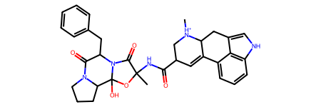
Let’s start by loading our “template” file with bond orders. It can be a SMILES string, MOL2, SDF file or anything supported by RDKit.
from rdkit import Chem

template = Chem.MolFromSmiles(
    "C[NH+]1CC(C(=O)NC2(C)OC3(O)C4CCCN4C(=O)C(Cc4ccccc4)N3C2=O)C=C2c3cccc4[nH]cc(c34)CC21"
)
template
Next, we’ll use the PDBQT supplier which loads each file from a list of paths, and assigns bond orders and charges using the template.
# load list of ligands
pdbqt_files = sorted(plf.datafiles.datapath.glob("vina/*.pdbqt"))
pdbqt_files
[PosixPath('/home/docs/checkouts/readthedocs.org/user_builds/prolif/checkouts/latest/prolif/data/vina/vina_output_ligand_1.pdbqt'),
 PosixPath('/home/docs/checkouts/readthedocs.org/user_builds/prolif/checkouts/latest/prolif/data/vina/vina_output_ligand_2.pdbqt'),
 PosixPath('/home/docs/checkouts/readthedocs.org/user_builds/prolif/checkouts/latest/prolif/data/vina/vina_output_ligand_3.pdbqt'),
 PosixPath('/home/docs/checkouts/readthedocs.org/user_builds/prolif/checkouts/latest/prolif/data/vina/vina_output_ligand_4.pdbqt'),
 PosixPath('/home/docs/checkouts/readthedocs.org/user_builds/prolif/checkouts/latest/prolif/data/vina/vina_output_ligand_5.pdbqt'),
 PosixPath('/home/docs/checkouts/readthedocs.org/user_builds/prolif/checkouts/latest/prolif/data/vina/vina_output_ligand_6.pdbqt'),
 PosixPath('/home/docs/checkouts/readthedocs.org/user_builds/prolif/checkouts/latest/prolif/data/vina/vina_output_ligand_7.pdbqt'),
 PosixPath('/home/docs/checkouts/readthedocs.org/user_builds/prolif/checkouts/latest/prolif/data/vina/vina_output_ligand_8.pdbqt'),
 PosixPath('/home/docs/checkouts/readthedocs.org/user_builds/prolif/checkouts/latest/prolif/data/vina/vina_output_ligand_9.pdbqt')]
pose_iterable = plf.pdbqt_supplier(pdbqt_files, template)
Fingerprint generation#
We can now generate a fingerprint. By default, ProLIF will calculate the following interactions: Hydrophobic, HBDonor, HBAcceptor, PiStacking, Anionic, Cationic, CationPi, PiCation, VdWContact. You can list all interactions that are available with the following command:
plf.Fingerprint.list_available()
['Anionic',
 'CationPi',
 'Cationic',
 'EdgeToFace',
 'FaceToFace',
 'HBAcceptor',
 'HBDonor',
 'Hydrophobic',
 'ImplicitHBAcceptor',
 'ImplicitHBDonor',
 'MetalAcceptor',
 'MetalDonor',
 'PiCation',
 'PiStacking',
 'VdWContact',
 'XBAcceptor',
 'XBDonor']
Tip
To perform an analysis of water-mediated interactions, consider this tutorial.
Tip
The default fingerprint will only keep track of the first group of atoms that satisfied the constraints per interaction type and residue pair.
If you want to keep track of all possible interactions to generate a count-fingerprint (e.g. when there are two atoms in the ligand that make an HBond-donor interaction with residue X), use plf.Fingerprint(count=True).
This is also quite useful for visualization purposes as you can then display the atom pair that has the shortest distance which will look more accurate.
This fingerprint type is however a bit slower to compute.
# use default interactions
fp = plf.Fingerprint()
# run on your poses
fp.run_from_iterable(pose_iterable, protein_mol)
<prolif.fingerprint.Fingerprint: 9 interactions: ['Hydrophobic', 'HBDonor', 'HBAcceptor', 'PiStacking', 'Anionic', 'Cationic', 'CationPi', 'PiCation', 'VdWContact'] at 0x7a5039c121d0>
Tip
The run_from_iterable method will automatically select residues that are close to the ligand (6.0 Å) when computing the fingerprint. You can modify the 6.0 Å cutoff by specifying plf.Fingerprint(vicinity_cutoff=7.0), but this is only useful if you decide to change the distance parameters for an interaction class (see in the advanced section of the tutorials).
Alternatively, you can pass a list of residues like so:
fp.run_from_iterable(<other parameters>, residues=["TYR38.A", "ASP129.A"])
You can save the fingerprint object with fp.to_pickle and reload it later with Fingerprint.from_pickle:
fp.to_pickle("fingerprint.pkl")
fp = plf.Fingerprint.from_pickle("fingerprint.pkl")
Analysis#
Once the execution is done, you can access the results through fp.ifp which is a nested dictionary:
pose_index = 0
ligand_residue = "LIG1.G"
protein_residue = "ASP129.A"

fp.ifp[pose_index][(ligand_residue, protein_residue)]
{'HBDonor': ({'indices': {'ligand': (20, 44), 'protein': (8,)},
   'parent_indices': {'ligand': (20, 44), 'protein': (1489,)},
   'distance': 3.0217454547036415,
   'DHA_angle': 148.56916365119588},),
 'Cationic': ({'indices': {'ligand': (20,), 'protein': (8,)},
   'parent_indices': {'ligand': (20,), 'protein': (1489,)},
   'distance': 3.0217454547036415},),
 'VdWContact': ({'indices': {'ligand': (20,), 'protein': (8,)},
   'parent_indices': {'ligand': (20,), 'protein': (1489,)},
   'distance': 3.0217454547036415},)}
While this contains all the details about the different interactions that were detected, it’s not the easiest thing to digest.
The best way to analyse our results is to export the interaction fingerprint to a Pandas DataFrame. You can read more about pandas in their user_guide.
df = fp.to_dataframe(index_col="Pose")
# show only the 5 first poses
df.head(5)
| ligand | LIG1.G | ||||||||||||||||||||
|---|---|---|---|---|---|---|---|---|---|---|---|---|---|---|---|---|---|---|---|---|---|
| protein | TYR38.A | TYR109.A | TRP125.A | LEU126.A | ... | MET337.B | PRO338.B | PHE346.B | LEU348.B | PHE351.B | ASP352.B | THR355.B | TYR359.B | ||||||||
| interaction | Hydrophobic | HBAcceptor | VdWContact | Hydrophobic | PiStacking | VdWContact | Hydrophobic | VdWContact | Hydrophobic | VdWContact | ... | VdWContact | VdWContact | Hydrophobic | Hydrophobic | VdWContact | Hydrophobic | VdWContact | VdWContact | VdWContact | Hydrophobic |
| Pose | |||||||||||||||||||||
| 0 | False | False | False | False | False | False | False | False | False | False | ... | True | False | False | False | False | True | True | False | False | False |
| 1 | False | False | False | False | False | False | False | False | True | True | ... | True | False | False | False | False | True | False | True | True | False |
| 2 | False | False | False | False | False | False | False | False | True | True | ... | False | False | False | False | False | False | False | True | True | False |
| 3 | False | False | True | False | False | False | False | False | False | False | ... | False | False | False | False | False | True | True | False | True | False |
| 4 | True | True | True | False | False | False | False | False | False | False | ... | False | True | True | True | True | True | True | False | False | False |
5 rows × 48 columns
Troubleshooting
If the dataframe only shows VdWContact interactions and nothing else, you may have a skipped the protein preparation step for protein PDB file: either all bonds should be explicit, or none of them.
If you only have partial bonds in your PDB file, MDAnalysis won’t trigger the bond guessing algorithm so your protein is essentially a point cloud that can’t match with any of the atom selections specified by interactions other than VdW.
To fix this, simply add the following line after creating a Universe from your protein file
with MDAnalysis:
u.atoms.guess_bonds()
and rerun the rest of the notebook.
Here are some common pandas snippets to extract useful information from the fingerprint table.
Important
Make sure to remove the .head(5) at the end of the commands to display the results for all the frames.
# hide an interaction type (Hydrophobic)
df.drop("Hydrophobic", level="interaction", axis=1).head(5)
| ligand | LIG1.G | ||||||||||||||||||||
|---|---|---|---|---|---|---|---|---|---|---|---|---|---|---|---|---|---|---|---|---|---|
| protein | TYR38.A | TYR109.A | TRP125.A | LEU126.A | ASP129.A | ILE130.A | ... | PHE330.B | PHE331.B | SER334.B | MET337.B | PRO338.B | LEU348.B | PHE351.B | ASP352.B | THR355.B | |||||
| interaction | HBAcceptor | VdWContact | PiStacking | VdWContact | VdWContact | VdWContact | HBDonor | Cationic | VdWContact | VdWContact | ... | PiStacking | VdWContact | VdWContact | VdWContact | VdWContact | VdWContact | VdWContact | VdWContact | VdWContact | VdWContact |
| Pose | |||||||||||||||||||||
| 0 | False | False | False | False | False | False | True | True | True | False | ... | False | True | True | False | True | False | False | True | False | False |
| 1 | False | False | False | False | False | True | False | False | False | True | ... | False | True | False | True | True | False | False | False | True | True |
| 2 | False | False | False | False | False | True | False | False | False | True | ... | False | True | False | True | False | False | False | False | True | True |
| 3 | False | True | False | False | False | False | True | False | True | True | ... | False | True | False | False | False | False | False | True | False | True |
| 4 | True | True | False | False | False | False | False | False | False | False | ... | True | True | False | True | False | True | True | True | False | False |
5 rows × 33 columns
# show only one protein residue (ASP129.A)
df.xs("ASP129.A", level="protein", axis=1).head(5)
| ligand | LIG1.G | ||
|---|---|---|---|
| interaction | HBDonor | Cationic | VdWContact |
| Pose | |||
| 0 | True | True | True |
| 1 | False | False | False |
| 2 | False | False | False |
| 3 | True | False | True |
| 4 | False | False | False |
# show only an interaction type (PiStacking)
df.xs("PiStacking", level="interaction", axis=1).head(5)
| ligand | LIG1.G | |
|---|---|---|
| protein | TYR109.A | PHE330.B |
| Pose | ||
| 0 | False | False |
| 1 | False | False |
| 2 | False | False |
| 3 | False | False |
| 4 | False | True |
# percentage of poses where each interaction is present
(df.mean().sort_values(ascending=False).to_frame(name="%").T * 100)
| ligand | LIG1.G | ||||||||||||||||||||
|---|---|---|---|---|---|---|---|---|---|---|---|---|---|---|---|---|---|---|---|---|---|
| protein | VAL201.A | PHE330.B | VAL201.A | PHE351.B | VAL201.A | VAL200.A | MET337.B | VAL200.A | ... | PHE330.B | TYR38.A | ASN202.A | GLN189.A | ARG188.A | PRO184.A | TRP125.A | TYR109.A | TYR359.B | |||
| interaction | VdWContact | VdWContact | Hydrophobic | Hydrophobic | Hydrophobic | VdWContact | HBAcceptor | VdWContact | Hydrophobic | Hydrophobic | ... | PiStacking | HBAcceptor | HBAcceptor | VdWContact | VdWContact | VdWContact | Hydrophobic | PiStacking | Hydrophobic | Hydrophobic |
| % | 100.0 | 77.777778 | 66.666667 | 66.666667 | 66.666667 | 55.555556 | 55.555556 | 55.555556 | 55.555556 | 44.444444 | ... | 11.111111 | 11.111111 | 11.111111 | 11.111111 | 11.111111 | 11.111111 | 11.111111 | 11.111111 | 11.111111 | 11.111111 |
1 rows × 48 columns
# same but we regroup all interaction types
(
    df.T.groupby(level=["ligand", "protein"])
    .sum()
    .T.astype(bool)
    .mean()
    .sort_values(ascending=False)
    .to_frame(name="%")
    .T
    * 100
)
| ligand | LIG1.G | ||||||||||||||||||||
|---|---|---|---|---|---|---|---|---|---|---|---|---|---|---|---|---|---|---|---|---|---|
| protein | VAL201.A | PHE330.B | VAL200.A | PHE351.B | MET337.B | ILE130.A | THR355.B | TYR38.A | ASP129.A | TYR208.A | ... | PHE331.B | TYR109.A | TRP125.A | TYR359.B | ARG188.A | PRO338.B | ASN202.A | PHE346.B | GLN189.A | PRO184.A |
| % | 100.0 | 88.888889 | 66.666667 | 66.666667 | 55.555556 | 44.444444 | 44.444444 | 44.444444 | 44.444444 | 44.444444 | ... | 22.222222 | 22.222222 | 22.222222 | 11.111111 | 11.111111 | 11.111111 | 11.111111 | 11.111111 | 11.111111 | 11.111111 |
1 rows × 27 columns
# percentage of poses where PiStacking interactions are present, by residue
(
    df.xs("PiStacking", level="interaction", axis=1)
    .mean()
    .sort_values(ascending=False)
    .to_frame(name="%")
    .T
    * 100
)
| ligand | LIG1.G | |
|---|---|---|
| protein | TYR109.A | PHE330.B |
| % | 11.111111 | 11.111111 |
# percentage of poses where interactions with PHE330 occur, by interaction type
(
    df.xs("PHE330.B", level="protein", axis=1)
    .mean()
    .sort_values(ascending=False)
    .to_frame(name="%")
    .T
    * 100
)
| ligand | LIG1.G | ||
|---|---|---|---|
| interaction | VdWContact | Hydrophobic | PiStacking |
| % | 77.777778 | 66.666667 | 11.111111 |
# percentage of poses where each interaction type is present
(
    df.T.groupby(level="interaction")
    .sum()
    .T.astype(bool)
    .mean()
    .sort_values(ascending=False)
    .to_frame(name="%")
    .T
    * 100
)
| interaction | Hydrophobic | VdWContact | HBAcceptor | HBDonor | Cationic | PiStacking |
|---|---|---|---|---|---|---|
| % | 100.0 | 100.0 | 77.777778 | 55.555556 | 33.333333 | 22.222222 |
# 10 residues most frequently interacting with the ligand
(
    df.T.groupby(level=["ligand", "protein"])
    .sum()
    .T.astype(bool)
    .mean()
    .sort_values(ascending=False)
    .head(10)
    .to_frame("%")
    .T
    * 100
)
| ligand | LIG1.G | |||||||||
|---|---|---|---|---|---|---|---|---|---|---|
| protein | VAL201.A | PHE330.B | VAL200.A | PHE351.B | MET337.B | ILE130.A | THR355.B | TYR38.A | ASP129.A | TYR208.A |
| % | 100.0 | 88.888889 | 66.666667 | 66.666667 | 55.555556 | 44.444444 | 44.444444 | 44.444444 | 44.444444 | 44.444444 |
You can compute a Tanimoto similarity between poses:
# Tanimoto similarity between the first frame and the rest
from rdkit import DataStructs

bitvectors = fp.to_bitvectors()
tanimoto_sims = DataStructs.BulkTanimotoSimilarity(bitvectors[0], bitvectors)
tanimoto_sims
[1.0,
 0.2962962962962963,
 0.17857142857142858,
 0.2608695652173913,
 0.2692307692307692,
 0.631578947368421,
 0.24,
 0.36363636363636365,
 0.18518518518518517]
Comparing docking poses with a reference ligand#
If you have a reference ligand that you wish to use for comparison with your docking poses, you can do so the following way:
Important
Just like for the protein, you reference ligand must contain explicit hydrogens. If the reference comes from a PDB file, you could use PyMOL to add hydrogens to it and export the prepared reference.
# load the reference
ref = mda.Universe(plf.datafiles.datapath / "vina" / "lig.pdb")
ref_mol = plf.Molecule.from_mda(ref)

# generate IFP for the reference
fp_ref = plf.Fingerprint(list(fp.interactions))
fp_ref.run_from_iterable([ref_mol], protein_mol)
df_ref = fp_ref.to_dataframe(index_col="Pose")

# set the "pose index" to -1
df_ref.rename(index={0: -1}, inplace=True)
# set the ligand name to be the same as poses
df_ref.rename(columns={str(ref_mol[0].resid): df.columns.levels[0][0]}, inplace=True)
df_ref
| ligand | LIG1.G | ||||||||||||||||||||
|---|---|---|---|---|---|---|---|---|---|---|---|---|---|---|---|---|---|---|---|---|---|
| protein | ASP129.A | ILE130.A | CYS133.A | VAL200.A | VAL201.A | SER212.A | ... | THR213.A | ALA216.A | PHE330.B | PHE331.B | MET337.B | PHE351.B | ASP352.B | |||||||
| interaction | HBDonor | Cationic | VdWContact | Hydrophobic | Hydrophobic | VdWContact | Hydrophobic | HBAcceptor | VdWContact | HBDonor | ... | VdWContact | VdWContact | Hydrophobic | VdWContact | Hydrophobic | PiStacking | VdWContact | Hydrophobic | Hydrophobic | VdWContact |
| Pose | |||||||||||||||||||||
| -1 | True | True | True | True | True | True | True | True | True | True | ... | True | True | True | True | True | True | True | True | True | True |
1 rows × 21 columns
# concatenate both dataframes
import pandas as pd

df_ref_poses = (
    pd.concat([df_ref, df])
    .fillna(False)
    .sort_index(
        axis=1,
        level=1,
        key=lambda index: [plf.ResidueId.from_string(x) for x in index],
    )
)
df_ref_poses
/tmp/ipykernel_1203/974255909.py:6: FutureWarning: Downcasting object dtype arrays on .fillna, .ffill, .bfill is deprecated and will change in a future version. Call result.infer_objects(copy=False) instead. To opt-in to the future behavior, set `pd.set_option('future.no_silent_downcasting', True)`
  .fillna(False)
| ligand | LIG1.G | ||||||||||||||||||||
|---|---|---|---|---|---|---|---|---|---|---|---|---|---|---|---|---|---|---|---|---|---|
| protein | TYR38.A | TYR109.A | TRP125.A | LEU126.A | ... | MET337.B | PRO338.B | PHE346.B | LEU348.B | PHE351.B | ASP352.B | THR355.B | TYR359.B | ||||||||
| interaction | HBAcceptor | Hydrophobic | VdWContact | Hydrophobic | PiStacking | VdWContact | Hydrophobic | VdWContact | Hydrophobic | VdWContact | ... | VdWContact | VdWContact | Hydrophobic | Hydrophobic | VdWContact | Hydrophobic | VdWContact | VdWContact | VdWContact | Hydrophobic |
| Pose | |||||||||||||||||||||
| -1 | False | False | False | False | False | False | False | False | False | False | ... | False | False | False | False | False | True | False | True | False | False |
| 0 | False | False | False | False | False | False | False | False | False | False | ... | True | False | False | False | False | True | True | False | False | False |
| 1 | False | False | False | False | False | False | False | False | True | True | ... | True | False | False | False | False | True | False | True | True | False |
| 2 | False | False | False | False | False | False | False | False | True | True | ... | False | False | False | False | False | False | False | True | True | False |
| 3 | False | False | True | False | False | False | False | False | False | False | ... | False | False | False | False | False | True | True | False | True | False |
| 4 | True | True | True | False | False | False | False | False | False | False | ... | False | True | True | True | True | True | True | False | False | False |
| 5 | False | False | False | False | False | False | False | False | False | False | ... | False | False | False | False | False | False | False | True | False | False |
| 6 | False | False | True | True | True | True | True | True | False | False | ... | True | False | False | False | True | True | True | False | True | True |
| 7 | False | False | True | False | False | True | False | True | False | False | ... | True | False | False | False | True | True | True | False | False | False |
| 8 | False | False | False | False | False | False | False | False | True | True | ... | False | False | False | False | False | False | False | False | False | False |
10 rows × 52 columns
We can now calculate the Tanimoto similarity between our reference ligand and the docking poses:
bitvectors = plf.to_bitvectors(df_ref_poses)
tanimoto_sims = DataStructs.BulkTanimotoSimilarity(bitvectors[0], bitvectors[1:])
tanimoto_sims
[0.5416666666666666,
 0.3333333333333333,
 0.3103448275862069,
 0.25925925925925924,
 0.22580645161290322,
 0.5652173913043478,
 0.125,
 0.25,
 0.1935483870967742]
Visualisation#
There are a few different options builtin when it comes to visualisation.
You can start by plotting the interactions over time:
# %matplotlib ipympl

fp.plot_barcode(xlabel="Pose")
<Axes: xlabel='Pose'>

Tip
If you uncomment %matplotlib ipympl at the top of the above cell, you should be able to see an interactive version of the plot.
You can also display the interactions in a 2D interactive diagram:
view = fp.plot_lignetwork(pose_iterable[0])
view
This diagram is interactive, you can:
zoom and pan,
move residues around,
click on the legend to display or hide types of residues or interactions,
hover an interaction line to display the distance.
Note
After arranging the residues to your liking, you can save the plot as a PNG image with:
view.save_png()
Note that this only works in notebooks and cannot be used in regular Python scripts.
You can generate 2 types of diagram with this function, controlled by the kind argument:
frame: shows a single specific docking pose (specified withframe, corresponds to thePoseindex in the dataframe).aggregate(default): the interactions from all poses are grouped and displayed. An optionalthresholdparameter controls the minimum frequency required for an interaction to be displayed (default0.3, meaning that interactions occuring in less than 30% of poses will be hidden). The width of interactions is linked to the frequency.
Showing a specific pose:
pose_index = 0
view = fp.plot_lignetwork(pose_iterable[pose_index], kind="frame", frame=pose_index)
view
Up to now we’ve only been using the default fingerprint generator, but you can optionally enable the count parameter to enumerate all occurences of an interaction (the default fingerprint generator will stop at the first occurence), and then display all of them by specifying display_all=True:
fp_count = plf.Fingerprint(count=True)
fp_count.run_from_iterable(pose_iterable, protein_mol)
view = fp_count.plot_lignetwork(
    pose_iterable[pose_index], kind="frame", frame=pose_index, display_all=True
)
view
You can also visualize this information in 3D:
view = fp_count.plot_3d(
    pose_iterable[pose_index], protein_mol, frame=pose_index, display_all=False
)
view
3Dmol.js failed to load for some reason. Please check your browser console for error messages.
<prolif.plotting.complex3d.Complex3D at 0x7a50309ec190>
As in the lignetwork plot, you can hover atoms and interactions to display more information.
The advantage of using a count fingerprint in that case is that it will automatically select the interaction occurence with the shortest distance for a more intuitive visualization.
Once you’re satisfied with the orientation, you can export the view as a PNG image with:
view.save_png()
Note that this only works in notebooks and cannot be used in regular Python scripts.
You can also compare two different poses on the same view, and the protein residues that have different interactions in the other pose or are missing will be highlighted in magenta:
from prolif.plotting.complex3d import Complex3D

pose_index = 0
comp3D = Complex3D.from_fingerprint(
    fp, pose_iterable[pose_index], protein_mol, frame=pose_index
)

pose_index = 4
other_comp3D = Complex3D.from_fingerprint(
    fp, pose_iterable[pose_index], protein_mol, frame=pose_index
)

view = comp3D.compare(other_comp3D)
view
3Dmol.js failed to load for some reason. Please check your browser console for error messages.
<prolif.plotting.complex3d.Complex3D at 0x7a5030a21150>
You could also superimpose them:
view = comp3D.display()
# other_comp3D will be displayed in green
other_comp3D.LIGAND_STYLE["stick"]["colorscheme"] = "greenCarbon"
other_comp3D._populate_view(view)
view
3Dmol.js failed to load for some reason. Please check your browser console for error messages.
<prolif.plotting.complex3d.Complex3D at 0x7a5030a21150>