Ligand-protein MD

This tutorial showcases how to use ProLIF to generate an interaction fingerprint for a ligand-protein complex from an MD simulation.

ProLIF uses MDAnalysis to process MD simulations, as it supports many file formats and is inter-operable with RDKit (which ProLIF uses under the hood to implement the different types of interactions). To learn more on how to use MDAnalysis, you can find their user guide here.

We will use 3 objects from the MDAnalysis library:

• The Universe which bundles the atoms and bonds of your system with the coordinates in your trajectory.

• The AtomGroup which is a collection of atoms that you can define by applying a selection on the Universe.

• The trajectory (or most often a subset of it) to know which frames to process.

Important

For convenience, the topology and trajectory files for this tutorial are included with the ProLIF installation, and you can access the path to both files through prolif.datafiles.TOP and prolif.datafiles.TRAJ respectively. Remember to switch these with the actual paths to your inputs outside of this tutorial.

Tip

At the top of the page you can find links to either download this notebook or run it in Google Colab. You can install the dependencies for the tutorials with the command:

pip install prolif[tutorials]

Preparation

Let’s start by importing MDAnalysis and ProLIF to read our tutorial files, and create selections for the ligand and protein:

import MDAnalysis as mda
import prolif as plf

# load topology and trajectory
u = mda.Universe(plf.datafiles.TOP, plf.datafiles.TRAJ)

# create selections for the ligand and protein
ligand_selection = u.select_atoms("resname LIG")
protein_selection = u.select_atoms("protein")
ligand_selection, protein_selection

(<AtomGroup with 79 atoms>, <AtomGroup with 4988 atoms>)

MDAnalysis should automatically recognize the file type that you’re using from its extension.

Note

Click here to learn more about loading files with MDAnalysis, and here to learn more about their atom selection language.

In our case the protein is of reasonable size, but if you’re working with a very large system, to save some time and memory it may be wise to restrict the protein selection to a sphere around the ligand:

protein_selection = u.select_atoms(
    "protein and byres around 20.0 group ligand", ligand=ligand_selection
)
protein_selection

<AtomGroup with 3311 atoms>

Depending on your system, it may be of interest to also include water molecules in the protein selection. There are none in this tutorial example but something like this could be used:

protein_selection = u.select_atoms(
    "(protein or resname WAT) and byres around 20.0 group ligand",
    ligand=ligand_selection,
)
protein_selection

<AtomGroup with 3311 atoms>

Next, lets make sure that our ligand was correctly read by MDAnalysis.

Important

This next step is crucial if you’re loading a structure from a file that doesn’t explicitely contain bond orders and formal charges, such as a PDB file or most MD trajectory files. MDAnalysis will infer those from the atoms connectivity, which requires all atoms including hydrogens to be present in the input file.

Since ProLIF molecules are built on top of RDKit, we can use RDKit functions to display molecules. Let’s have a quick look at our ligand:

# create a molecule from the MDAnalysis selection
ligand_mol = plf.Molecule.from_mda(ligand_selection)
# display
plf.display_residues(ligand_mol, size=(400, 200))

We can do the same for the residues in the protein (only showing the first 20 to keep the notebook short):

protein_mol = plf.Molecule.from_mda(protein_selection)
# remove the `slice(20)` part to show all residues
plf.display_residues(protein_mol, slice(20))

Troubleshooting

If one of the two molecules was not processed correctly, it might be because your input file does not contain bond information. If that’s the case, please add this snippet right after creating your selections:

ligand_selection.guess_bonds()
protein_selection.guess_bonds()

In some cases, some atomic clashes may be incorrectly classified as bonds and will prevent the conversion of MDAnalysis molecules to RDKit. Since MDAnalysis uses van der Waals radii for bond detection, one can modify the default radii that are used:

protein_selection.guess_bonds(vdwradii={"H": 1.05, "O": 1.48})

Fingerprint generation

Everything looks good, we can now generate a fingerprint. By default, ProLIF will calculate the following interactions: Hydrophobic, HBDonor, HBAcceptor, PiStacking, Anionic, Cationic, CationPi, PiCation, VdWContact. You can list all interactions that are available with the following command:

plf.Fingerprint.list_available()

['Anionic',
 'CationPi',
 'Cationic',
 'EdgeToFace',
 'FaceToFace',
 'HBAcceptor',
 'HBDonor',
 'Hydrophobic',
 'MetalAcceptor',
 'MetalDonor',
 'PiCation',
 'PiStacking',
 'VdWContact',
 'XBAcceptor',
 'XBDonor']

Tip

The default fingerprint will only keep track of the first group of atoms that satisfied the constraints per interaction type and residue pair.

If you want to keep track of all possible interactions to generate a count-fingerprint (e.g. when there are two atoms in the ligand that make an HBond-donor interaction with residue X), use plf.Fingerprint(count=True). This is also quite useful for visualization purposes as you can then display the atom pair that has the shortest distance which will look more accurate. This fingerprint type is however a bit slower to compute.

# use default interactions
fp = plf.Fingerprint()
# run on a slice of the trajectory frames: from begining to end with a step of 10
fp.run(u.trajectory[::10], ligand_selection, protein_selection)

<prolif.fingerprint.Fingerprint: 9 interactions: ['Hydrophobic', 'HBAcceptor', 'HBDonor', 'Cationic', 'Anionic', 'CationPi', 'PiCation', 'PiStacking', 'VdWContact'] at 0x7f5ecc453450>

Tip

The run method will automatically select residues that are close to the ligand (6.0 Å) when computing the fingerprint. You can modify the 6.0 Å cutoff by specifying plf.Fingerprint(vicinity_cutoff=7.0), but this is only useful if you decide to change the distance parameters for an interaction class (see in the advanced section of the tutorials).

Alternatively, you can pass a list of residues like so:

fp.run(<other parameters>, residues=["TYR38.A", "ASP129.A"])

You can save the fingerprint object with fp.to_pickle and reload it later with Fingerprint.from_pickle:

fp.to_pickle("fingerprint.pkl")
fp = plf.Fingerprint.from_pickle("fingerprint.pkl")

Analysis

Once the execution is done, you can access the results through fp.ifp which is a nested dictionary:

frame_number = 0
ligand_residue = "LIG1.G"
protein_residue = "ASP129.A"

fp.ifp[frame_number][(ligand_residue, protein_residue)]

{'HBDonor': ({'indices': {'ligand': (13, 52), 'protein': (8,)},
   'parent_indices': {'ligand': (13, 52), 'protein': (1199,)},
   'distance': 2.7534162113079534,
   'DHA_angle': 158.09471525304645},),
 'Cationic': ({'indices': {'ligand': (13,), 'protein': (8,)},
   'parent_indices': {'ligand': (13,), 'protein': (1199,)},
   'distance': 2.7534162113079534},),
 'VdWContact': ({'indices': {'ligand': (8,), 'protein': (8,)},
   'parent_indices': {'ligand': (8,), 'protein': (1199,)},
   'distance': 3.1985935380346855},)}

While this contains all the details about the different interactions that were detected, it’s not the easiest thing to digest.

The best way to analyse our results is to export the interaction fingerprint to a Pandas DataFrame. You can read more about pandas in their user_guide.

df = fp.to_dataframe()
# show only the 10 first frames
df.head(10)

ligand	LIG1.G
protein	TYR38.A		TYR109.A		THR110.A	TRP125.A		LEU126.A		ASP129.A	...	ALA343.B	LEU348.B		PHE351.B			ASP352.B		THR355.B	TYR359.B
interaction	Hydrophobic	VdWContact	Hydrophobic	VdWContact	Hydrophobic	Hydrophobic	VdWContact	Hydrophobic	VdWContact	Hydrophobic	...	Hydrophobic	Hydrophobic	VdWContact	Hydrophobic	PiStacking	VdWContact	Hydrophobic	VdWContact	VdWContact	VdWContact
Frame
0	False	False	True	False	False	True	False	True	False	False	...	False	False	False	True	False	False	False	True	False	False
10	False	False	True	True	False	True	False	True	False	False	...	True	False	False	True	False	False	False	False	True	True
20	False	False	True	True	False	True	True	True	True	False	...	True	False	False	True	False	False	False	False	False	True
30	True	False	True	False	False	True	True	True	False	False	...	True	False	False	True	False	True	False	False	True	True
40	False	False	True	False	True	True	True	True	True	False	...	False	False	False	True	False	False	False	False	False	False
50	True	False	True	True	False	False	False	True	False	True	...	False	False	False	True	False	True	False	False	True	True
60	False	False	True	False	False	False	False	True	False	False	...	False	False	False	True	False	True	False	False	False	False
70	False	False	True	True	False	True	False	True	False	False	...	False	True	False	True	True	False	False	False	False	True
80	False	False	True	False	False	True	False	True	False	False	...	False	True	False	True	False	True	False	False	False	False
90	False	False	False	False	False	True	False	False	False	False	...	False	True	True	True	False	True	True	True	False	False

10 rows × 63 columns

Here are some common pandas snippets to extract useful information from the fingerprint table.

Important

Make sure to remove the .head(5) at the end of the commands to display the results for all the frames.

# hide an interaction type (Hydrophobic)
df.drop("Hydrophobic", level="interaction", axis=1).head(5)

ligand	LIG1.G
protein	TYR38.A	TYR109.A	TRP125.A	LEU126.A	ASP129.A			ILE130.A	CYS133.A	THR134.A	...	PHE331.B	SER334.B	MET337.B	PRO338.B	LEU348.B	PHE351.B		ASP352.B	THR355.B	TYR359.B
interaction	VdWContact	VdWContact	VdWContact	VdWContact	HBDonor	Cationic	VdWContact	VdWContact	VdWContact	HBDonor	...	VdWContact	VdWContact	VdWContact	VdWContact	VdWContact	PiStacking	VdWContact	VdWContact	VdWContact	VdWContact
Frame
0	False	False	False	False	True	True	True	False	False	False	...	True	False	False	False	False	False	False	True	False	False
10	False	True	False	False	True	True	True	False	False	False	...	True	False	False	False	False	False	False	False	True	True
20	False	True	True	True	True	True	True	True	True	False	...	False	False	False	False	False	False	False	False	False	True
30	False	False	True	False	True	True	True	True	False	False	...	False	False	False	False	False	False	True	False	True	True
40	False	False	True	True	True	True	True	True	False	False	...	False	False	False	False	False	False	False	False	False	False

5 rows × 37 columns

# show only one protein residue (ASP129.A)
df.xs("ASP129.A", level="protein", axis=1).head(5)

ligand	LIG1.G
interaction	Hydrophobic	HBDonor	Cationic	VdWContact
Frame
0	False	True	True	True
10	False	True	True	True
20	False	True	True	True
30	False	True	True	True
40	False	True	True	True

# show only an interaction type (PiStacking)
df.xs("PiStacking", level="interaction", axis=1).head(5)

ligand	LIG1.G
protein	PHE330.B	PHE331.B	PHE351.B
Frame
0	False	True	False
10	False	False	False
20	True	False	False
30	False	False	False
40	False	False	False

# percentage of the trajectory where each interaction is present
(df.mean().sort_values(ascending=False).to_frame(name="%").T * 100)

ligand	LIG1.G
protein	ASP129.A			VAL201.A	PHE351.B	CYS133.A	ILE130.A	PHE331.B	PHE330.B	VAL201.A	...	TRP125.A	CYS199.A	PHE330.B	THR209.A	MET337.B	ILE206.A	THR134.A		THR110.A	PRO338.B
interaction	VdWContact	Cationic	HBDonor	VdWContact	Hydrophobic	Hydrophobic	Hydrophobic	Hydrophobic	Hydrophobic	HBAcceptor	...	VdWContact	Hydrophobic	CationPi	VdWContact	VdWContact	VdWContact	VdWContact	HBDonor	Hydrophobic	VdWContact
%	100.0	100.0	100.0	100.0	100.0	96.0	96.0	96.0	96.0	92.0	...	12.0	8.0	8.0	8.0	8.0	8.0	4.0	4.0	4.0	4.0

1 rows × 63 columns

# same but we regroup all interaction types
(
    df.T.groupby(level=["ligand", "protein"])
    .sum()
    .T.astype(bool)
    .mean()
    .sort_values(ascending=False)
    .to_frame(name="%")
    .T
    * 100
)

ligand	LIG1.G
protein	ASP129.A	PHE351.B	VAL201.A	PHE330.B	PHE331.B	CYS133.A	ILE130.A	VAL200.A	ALA216.A	MET337.B	...	TYR359.B	THR355.B	ILE206.A	SER334.B	PRO338.B	CYS199.A	ALA343.B	VAL210.A	THR110.A	THR134.A
%	100.0	100.0	100.0	96.0	96.0	96.0	96.0	96.0	68.0	64.0	...	32.0	32.0	28.0	24.0	24.0	12.0	12.0	12.0	4.0	4.0

1 rows × 31 columns

# percentage of the trajectory where PiStacking interactions are present, by residue
(
    df.xs("PiStacking", level="interaction", axis=1)
    .mean()
    .sort_values(ascending=False)
    .to_frame(name="%")
    .T
    * 100
)

ligand	LIG1.G
protein	PHE351.B	PHE331.B	PHE330.B
%	36.0	20.0	12.0

# percentage of the trajectory where interactions with SER212 occur, by interaction type
(
    df.xs("SER212.A", level="protein", axis=1)
    .mean()
    .sort_values(ascending=False)
    .to_frame(name="%")
    .T
    * 100
)

ligand	LIG1.G
interaction	VdWContact	HBDonor
%	56.0	32.0

# percentage of the trajectory where each interaction type is present
(
    df.T.groupby(level="interaction")
    .sum()
    .T.astype(bool)
    .mean()
    .sort_values(ascending=False)
    .to_frame(name="%")
    .T
    * 100
)

interaction	Cationic	Hydrophobic	HBDonor	VdWContact	HBAcceptor	PiStacking	CationPi
%	100.0	100.0	100.0	100.0	92.0	60.0	8.0

# 10 residues most frequently interacting with the ligand
(
    df.T.groupby(level=["ligand", "protein"])
    .sum()
    .T.astype(bool)
    .mean()
    .sort_values(ascending=False)
    .head(10)
    .to_frame("%")
    .T
    * 100
)

ligand	LIG1.G
protein	ASP129.A	PHE351.B	VAL201.A	PHE330.B	PHE331.B	CYS133.A	ILE130.A	VAL200.A	ALA216.A	MET337.B
%	100.0	100.0	100.0	96.0	96.0	96.0	96.0	96.0	68.0	64.0

You can compute a Tanimoto similarity between frames:

# Tanimoto similarity between the first frame and the rest
from rdkit import DataStructs

bitvectors = fp.to_bitvectors()
tanimoto_sims = DataStructs.BulkTanimotoSimilarity(bitvectors[0], bitvectors)
tanimoto_sims

[1.0,
 0.6285714285714286,
 0.5,
 0.5833333333333334,
 0.6176470588235294,
 0.5405405405405406,
 0.65625,
 0.5714285714285714,
 0.6111111111111112,
 0.5588235294117647,
 0.42105263157894735,
 0.4444444444444444,
 0.40540540540540543,
 0.3783783783783784,
 0.43243243243243246,
 0.5,
 0.4594594594594595,
 0.6875,
 0.4864864864864865,
 0.5757575757575758,
 0.5833333333333334,
 0.5526315789473685,
 0.43243243243243246,
 0.5609756097560976,
 0.41025641025641024]

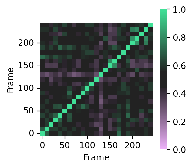
To compare binding modes in your trajectory, it’s possible to compute the entire similarity matrix:

import pandas as pd
import seaborn as sns
from matplotlib import pyplot as plt

# Tanimoto similarity matrix
bitvectors = fp.to_bitvectors()
similarity_matrix = []
for bv in bitvectors:
    similarity_matrix.append(DataStructs.BulkTanimotoSimilarity(bv, bitvectors))
similarity_matrix = pd.DataFrame(similarity_matrix, index=df.index, columns=df.index)

# display heatmap
fig, ax = plt.subplots(figsize=(3, 3), dpi=200)
colormap = sns.diverging_palette(
    300, 145, s=90, l=80, sep=30, center="dark", as_cmap=True
)
sns.heatmap(
    similarity_matrix,
    ax=ax,
    square=True,
    cmap=colormap,
    vmin=0,
    vmax=1,
    center=0.5,
    xticklabels=5,
    yticklabels=5,
)
ax.invert_yaxis()
plt.yticks(rotation="horizontal")
fig.patch.set_facecolor("white")

Visualisation

There are a few different options builtin when it comes to visualisation.

You can start by plotting the interactions over time:

# %matplotlib ipympl

fp.plot_barcode()

<Axes: xlabel='Frame'>

Tip

If you uncomment %matplotlib ipympl at the top of the above cell, you should be able to see an interactive version of the plot.

You can also display the interactions in a 2D interactive diagram:

fp.plot_lignetwork(ligand_mol)

This diagram is interactive, you can:

• zoom and pan,

• move residues around,

• click on the legend to display or hide types of residues or interactions,

• hover an interaction line to display the distance.

Note

It is not possible to export it as an image, but you can always take a screenshot.

You can generate 2 types of diagram with this function, controlled by the kind argument:

• frame: shows a single specific frame (specified with frame, corresponds to the frame number in the simulation).

• aggregate (default): the interactions from all frames are grouped and displayed. An optional threshold parameter controls the minimum frequency required for an interaction to be displayed (default 0.3, meaning that interactions occuring in less than 30% of frames will be hidden). The width of interactions is linked to the frequency.

Some more examples:

fp.plot_lignetwork(ligand_mol, threshold=0.0)

Up to now we’ve only been using the default fingerprint generator, but you can optionally enable the count parameter to enumerate all occurences of an interaction (the default fingerprint generator will stop at the first occurence), and then display all of them by specifying display_all=True:

fp_count = plf.Fingerprint(count=True)
fp_count.run(u.trajectory[0:1], ligand_selection, protein_selection)
fp_count.plot_lignetwork(ligand_mol, kind="frame", frame=0, display_all=True)

You can also visualize this information in 3D:

frame = 0
# seek specific frame
u.trajectory[frame]
ligand_mol = plf.Molecule.from_mda(ligand_selection)
protein_mol = plf.Molecule.from_mda(protein_selection)
# display
view = fp_count.plot_3d(ligand_mol, protein_mol, frame=frame, display_all=False)
view

3Dmol.js failed to load for some reason. Please check your browser console for error messages.

<py3Dmol.view at 0x7f5ec17df510>

As in the lignetwork plot, you can hover atoms and interactions to display more information.

The advantage of using a count fingerprint in that case is that it will automatically select the interaction occurence with the shortest distance for a more intuitive visualization.

Once you’re satisfied with the orientation, you can export the view as a PNG image with the following snippet:

from IPython.display import Javascript

Javascript(
    """
    var png = viewer_%s.pngURI()
    var a = document.createElement('a')
    a.href = png
    a.download = "prolif-3d.png"
    a.click()
    a.remove()
    """
    % view.uniqueid
)

You can also compare two different frames on the same view, and the protein residues that have different interactions in the other frame or are missing will be highlighted in magenta:

from prolif.plotting.complex3d import Complex3D

frame = 0
u.trajectory[frame]
ligand_mol = plf.Molecule.from_mda(ligand_selection)
protein_mol = plf.Molecule.from_mda(protein_selection)
comp3D = Complex3D.from_fingerprint(fp, ligand_mol, protein_mol, frame=frame)

frame = 120
u.trajectory[frame]
ligand_mol = plf.Molecule.from_mda(ligand_selection)
protein_mol = plf.Molecule.from_mda(protein_selection)
other_comp3D = Complex3D.from_fingerprint(fp, ligand_mol, protein_mol, frame=frame)

view = comp3D.compare(other_comp3D)
view

3Dmol.js failed to load for some reason. Please check your browser console for error messages.

<py3Dmol.view at 0x7f5ec14fe050>