Protein-protein MD#
This tutorial showcases how to use ProLIF to generate an interaction fingerprint for protein-protein interactions in an MD simulation.
ProLIF uses MDAnalysis to process MD simulations, as it supports many file formats and is inter-operable with RDKit (which ProLIF uses under the hood to implement the different types of interactions). To learn more on how to use MDAnalysis, you can find their user guide here.
We will use 3 objects from the MDAnalysis library:
The
Universewhich bundles the atoms and bonds of your system with the coordinates in your trajectory.The
AtomGroupwhich is a collection of atoms that you can define by applying a selection on theUniverse.The trajectory (or most often a subset of it) to know which frames to process.
Important
For convenience, the topology and trajectory files for this tutorial are included with the ProLIF installation, and you can access the path to both files through prolif.datafiles.TOP and prolif.datafiles.TRAJ respectively. Remember to switch these with the actual paths to your inputs outside of this tutorial.
Tip
At the top of the page you can find links to either download this notebook or run it in Google Colab. You can install the dependencies for the tutorials with the command:
pip install prolif[tutorials]
Preparation#
Let’s start by importing MDAnalysis and ProLIF to read our tutorial files, and create selections for the protein components. To keep the size of tutorial files short, we are going to reuse the same simulation as for the ligand-protein system, and decompose our protein in 2 virtual segments: one of the seven transmembrane domains of the GPCR, and the rest of the GPCR. In a real-world scenario this could be for example a peptide and a protein.
import MDAnalysis as mda
import prolif as plf

# load topology and trajectory
u = mda.Universe(plf.datafiles.TOP, plf.datafiles.TRAJ)

# create selections for both protein components
small_protein_selection = u.select_atoms("resid 119:152")
large_protein_selection = u.select_atoms(
    "protein and not group peptide", peptide=small_protein_selection
)
small_protein_selection, large_protein_selection
/home/docs/checkouts/readthedocs.org/user_builds/prolif/envs/latest/lib/python3.11/site-packages/MDAnalysis/topology/TPRParser.py:161: DeprecationWarning: 'xdrlib' is deprecated and slated for removal in Python 3.13
  import xdrlib
(<AtomGroup with 531 atoms>, <AtomGroup with 4457 atoms>)
MDAnalysis should automatically recognize the file type that you’re using from its extension.
Note
Click here to learn more about loading files with MDAnalysis, and here to learn more about their atom selection language.
In our case the protein is of reasonable size, but if you’re working with a very large system, to save some time and memory it may be wise to restrict the protein selection to a sphere around the peptide:
large_protein_selection = u.select_atoms(
    "protein and byres around 20.0 group peptide", peptide=small_protein_selection
)
large_protein_selection
<AtomGroup with 4122 atoms>
Important
Note that this will only select residues around 20Å of the ligand on the first frame. If your ligand or protein moves significantly during the simulation and moves outside of this 20Å sphere, it may be more relevant to perform this selection multiple times during the simulation to encompass all the relevant residues across the entire trajectory.
To this effect, you can use select_over_trajectory():
large_protein_selection = plf.select_over_trajectory(
    u,
    u.trajectory[::10],
    "protein and byres around 6.0 group peptide",
    peptide=small_protein_selection,
)
Depending on your system, it may be of interest to also include water molecules in the protein selection. There are none in this tutorial example but something like this could be used:
large_protein_selection = u.select_atoms(
    "(protein or resname WAT) and byres around 20.0 group peptide",
    peptide=small_protein_selection,
)
large_protein_selection
<AtomGroup with 4122 atoms>
Tip
To perform an analysis of water-mediated interactions, consider this tutorial.
Next, lets make sure that both components were correctly read by MDAnalysis.
Important
This next step is crucial if you’re loading a structure from a file that doesn’t explicitely contain bond orders and formal charges, such as a PDB file or most MD trajectory files. MDAnalysis will infer those from the atoms connectivity, which requires all atoms including hydrogens to be present in the input file.
Since ProLIF molecules are built on top of RDKit, we can use RDKit functions to display molecules. Let’s have a quick look at our protein selections. We’ll only show the first 20 residue to keep the notebook short, this should be enough to detect any compatibility problem between ProLIF/MDAnalysis and your input if any.
# create a molecule from the MDAnalysis selection
small_protein_mol = plf.Molecule.from_mda(small_protein_selection)

# display (remove `slice(20)` to show all residues)
plf.display_residues(small_protein_mol, slice(20))

We can do the same for the residues in the other protein selection:
# create a molecule from the MDAnalysis selection
large_protein_mol = plf.Molecule.from_mda(large_protein_selection)

# display (remove `slice(20)` to show all residues)
plf.display_residues(large_protein_mol, slice(20))

Troubleshooting
If one of the two molecules was not processed correctly, it might be because your input file does not contain bond information. If that’s the case, please add this snippet right after creating your selections:
small_protein_selection.guess_bonds()
large_protein_selection.guess_bonds()
In some cases, some atomic clashes may be incorrectly classified as bonds and will prevent the conversion of MDAnalysis molecules to RDKit. Since MDAnalysis uses van der Waals radii for bond detection, one can modify the default radii that are used:
small_protein_selection.guess_bonds(vdwradii={"H": 1.05, "O": 1.48})
Advanced usage
If you would like to ignore backbone interactions in the analysis, head over to the corresponding section of the advanced tutorial: Ignoring the protein backbone
Fingerprint generation#
Everything looks good, we can now generate a fingerprint. By default, ProLIF will calculate the following interactions: Hydrophobic, HBDonor, HBAcceptor, PiStacking, Anionic, Cationic, CationPi, PiCation, VdWContact. You can list all interactions that are available with the following command:
plf.Fingerprint.list_available()
['Anionic',
 'CationPi',
 'Cationic',
 'EdgeToFace',
 'FaceToFace',
 'HBAcceptor',
 'HBDonor',
 'Hydrophobic',
 'ImplicitHBAcceptor',
 'ImplicitHBDonor',
 'MetalAcceptor',
 'MetalDonor',
 'PiCation',
 'PiStacking',
 'VdWContact',
 'XBAcceptor',
 'XBDonor']
Tip
The default fingerprint will only keep track of the first group of atoms that satisfied the constraints per interaction type and residue pair.
If you want to keep track of all possible interactions to generate a count-fingerprint (e.g. when there are two atoms in the ligand that make an HBond-donor interaction with residue X), use plf.Fingerprint(count=True).
This is also quite useful for visualization purposes as you can then display the atom pair that has the shortest distance which will look more accurate.
This fingerprint type is however a bit slower to compute.
# ignore VdWContact and Hydrophobic interactions
fp = plf.Fingerprint(
    [
        "HBDonor",
        "HBAcceptor",
        "PiStacking",
        "PiCation",
        "CationPi",
        "Anionic",
        "Cationic",
    ]
)
# run on a slice of the trajectory frames: from begining to end with a step of 10
fp.run(u.trajectory[::10], small_protein_selection, large_protein_selection)
<prolif.fingerprint.Fingerprint: 7 interactions: ['HBDonor', 'HBAcceptor', 'PiStacking', 'PiCation', 'CationPi', 'Anionic', 'Cationic'] at 0x7b2ceaa3d190>
Note
See the Parallel processing section for details on how to control the number of processes used and the parallelization strategy.
Tip
The run method will automatically select residues that are close to the ligand (6.0 Å) when computing the fingerprint. You can modify the 6.0 Å cutoff by specifying plf.Fingerprint(vicinity_cutoff=7.0), but this is only useful if you decide to change the distance parameters for an interaction class (see in the advanced section of the tutorials).
Alternatively, you can pass a list of residues like so:
fp.run(<other parameters>, residues=["TYR38.A", "ASP129.A"])
You can save the fingerprint object with fp.to_pickle and reload it later with Fingerprint.from_pickle:
fp.to_pickle("fingerprint.pkl")
fp = plf.Fingerprint.from_pickle("fingerprint.pkl")
Analysis#
Once the execution is done, you can access the results through fp.ifp which is a nested dictionary:
frame_number = 0
residues = ("ASP129.A", "TYR359.B")

fp.ifp[frame_number][residues]
{'HBAcceptor': ({'indices': {'ligand': (9,), 'protein': (13, 14)},
   'parent_indices': {'ligand': (165,), 'protein': (3773, 3774)},
   'distance': 3.0682571478876968,
   'DHA_angle': 166.77312338568785},)}
Note
Internally, ProLIF uses ligand and protein as a naming convention for components, but it uses whatever was passed as the first selection in the fp.run call as the ligand and the second object as the protein.
While this contains all the details about the different interactions that were detected, it’s not the easiest thing to digest.
The best way to analyse our results is to export the interaction fingerprint to a Pandas DataFrame. You can read more about pandas in their user_guide.
df = fp.to_dataframe()
# show only the 10 first frames
df.head(10)
| ligand | GLN119.A | ... | ALA150.A | ILE151.A | THR152.A | ||||||||||||||||
|---|---|---|---|---|---|---|---|---|---|---|---|---|---|---|---|---|---|---|---|---|---|
| protein | GLN189.A | ALA190.A | ALA192.A | GLU194.A | VAL196.A | SER197.A | GLU198.A | ... | ALA154.A | ARG238.A | ALA154.A | ARG238.A | ASN245.A | ASP153.A | GLU234.A | ARG238.A | LYS241.A | ||||
| interaction | HBAcceptor | HBDonor | HBDonor | HBAcceptor | HBDonor | HBAcceptor | HBDonor | HBAcceptor | HBDonor | HBDonor | ... | HBAcceptor | HBAcceptor | HBAcceptor | HBAcceptor | HBAcceptor | HBDonor | HBAcceptor | HBDonor | HBAcceptor | HBAcceptor |
| Frame | |||||||||||||||||||||
| 0 | False | False | True | False | False | True | False | False | False | False | ... | False | False | False | False | False | False | False | False | False | False |
| 10 | False | False | False | False | False | False | False | False | False | False | ... | False | False | False | True | False | False | False | False | False | False |
| 20 | False | False | False | False | False | False | False | False | False | True | ... | False | False | False | True | False | False | True | False | True | False |
| 30 | False | False | False | False | False | False | False | False | False | False | ... | False | False | False | False | False | False | False | False | False | False |
| 40 | False | False | False | False | True | False | False | True | False | False | ... | False | False | True | True | False | False | False | False | False | False |
| 50 | False | False | False | False | False | False | False | False | False | True | ... | False | False | True | False | False | False | False | False | False | False |
| 60 | False | False | False | False | False | False | False | False | False | False | ... | False | False | False | False | False | False | False | False | False | False |
| 70 | False | False | False | False | False | False | False | False | False | False | ... | False | False | False | False | False | False | False | False | False | False |
| 80 | False | False | False | False | False | False | False | False | True | False | ... | True | False | False | False | False | True | False | False | False | False |
| 90 | False | True | False | True | False | False | False | False | False | False | ... | False | False | False | True | False | False | False | False | False | False |
10 rows × 52 columns
Here are some common pandas snippets to extract useful information from the fingerprint table.
Important
Make sure to remove the .head(5) at the end of the commands to display the results for all the frames.
# hide an interaction type (HBAcceptor)
df.drop("HBAcceptor", level="interaction", axis=1).head(5)
| ligand | GLN119.A | CYS122.A | ASP123.A | ... | THR131.A | CYS133.A | ASP146.A | ARG147.A | TRP149.A | THR152.A | |||||||||||
|---|---|---|---|---|---|---|---|---|---|---|---|---|---|---|---|---|---|---|---|---|---|
| protein | ALA190.A | ALA192.A | GLU194.A | VAL196.A | SER197.A | GLU198.A | GLY118.A | LYS191.A | ARG188.A | LYS191.A | ... | SER181.A | ALA216.A | ARG161.A | ALA84.A | GLU309.B | THR313.B | TYR157.A | ASP153.A | GLU234.A | |
| interaction | HBDonor | HBDonor | HBDonor | HBDonor | HBDonor | HBDonor | HBDonor | Anionic | Anionic | Anionic | ... | HBDonor | HBDonor | Anionic | HBDonor | HBDonor | Cationic | HBDonor | PiStacking | HBDonor | HBDonor |
| Frame | |||||||||||||||||||||
| 0 | False | True | False | False | False | False | True | False | False | False | ... | False | False | False | False | False | False | False | False | False | False |
| 10 | False | False | False | False | False | False | True | False | False | False | ... | False | False | False | False | False | False | False | False | False | False |
| 20 | False | False | False | False | False | True | True | False | False | True | ... | False | False | False | True | False | False | False | False | False | False |
| 30 | False | False | False | False | False | False | True | False | True | False | ... | False | False | True | False | False | False | False | False | False | False |
| 40 | False | False | True | False | False | False | True | False | False | True | ... | False | False | False | False | True | True | False | False | False | False |
5 rows × 24 columns
# show only one protein residue (LYS191.A)
df.xs("LYS191.A", level="protein", axis=1).head(5)
| ligand | CYS122.A | ASP123.A | |
|---|---|---|---|
| interaction | Anionic | HBAcceptor | Anionic |
| Frame | |||
| 0 | False | False | False |
| 10 | False | False | False |
| 20 | False | True | True |
| 30 | False | False | False |
| 40 | False | True | True |
# show only an interaction type (PiStacking)
df.xs("PiStacking", level="interaction", axis=1).head(5)
| ligand | TRP149.A |
|---|---|
| protein | TYR157.A |
| Frame | |
| 0 | False |
| 10 | False |
| 20 | False |
| 30 | False |
| 40 | False |
# percentage of the trajectory where each interaction is present
(df.mean().sort_values(ascending=False).to_frame(name="%").T * 100)
| ligand | HSD139.A | ASP129.A | ASP146.A | CYS122.A | TRP125.A | ASP146.A | ARG147.A | TRP149.A | ... | GLN119.A | TRP149.A | GLN119.A | ARG147.A | CYS122.A | HSD139.A | THR152.A | |||||
|---|---|---|---|---|---|---|---|---|---|---|---|---|---|---|---|---|---|---|---|---|---|
| protein | SER90.A | TYR359.B | TYR157.A | GLY118.A | VAL102.A | ARG161.A | GLU309.B | ASP153.A | ... | VAL196.A | GLU194.A | TYR157.A | SER197.A | GLU198.A | CYS199.A | ALA84.A | LYS191.A | TRP174.A | LYS241.A | ||
| interaction | HBAcceptor | HBAcceptor | HBAcceptor | HBDonor | HBDonor | HBAcceptor | Anionic | Cationic | HBDonor | HBAcceptor | ... | HBDonor | HBAcceptor | PiStacking | HBDonor | HBAcceptor | HBAcceptor | HBDonor | Anionic | HBAcceptor | HBAcceptor |
| % | 100.0 | 96.0 | 88.0 | 84.0 | 60.0 | 48.0 | 48.0 | 44.0 | 44.0 | 36.0 | ... | 4.0 | 4.0 | 4.0 | 4.0 | 4.0 | 4.0 | 4.0 | 4.0 | 4.0 | 4.0 |
1 rows × 52 columns
# same but we regroup all interaction types
(
    df.T.groupby(level=["ligand", "protein"])
    .sum()
    .T.astype(bool)
    .mean()
    .sort_values(ascending=False)
    .to_frame(name="%")
    .T
    * 100
)
| ligand | HSD139.A | ASP129.A | ASP146.A | CYS122.A | TRP125.A | ASP146.A | ARG147.A | TRP149.A | SER127.A | ASP123.A | ... | ALA150.A | THR152.A | SER136.A | ILE151.A | HSD139.A | ALA150.A | GLN119.A | CYS122.A | ARG147.A | GLN119.A |
|---|---|---|---|---|---|---|---|---|---|---|---|---|---|---|---|---|---|---|---|---|---|
| protein | SER90.A | TYR359.B | TYR157.A | GLY118.A | VAL102.A | ARG161.A | GLU309.B | ASP153.A | SER181.A | LYS191.A | ... | ALA154.A | ARG238.A | ASP95.A | ASN245.A | TRP174.A | ARG238.A | CYS199.A | LYS191.A | ALA84.A | SER197.A |
| % | 100.0 | 96.0 | 88.0 | 84.0 | 60.0 | 48.0 | 44.0 | 36.0 | 32.0 | 32.0 | ... | 4.0 | 4.0 | 4.0 | 4.0 | 4.0 | 4.0 | 4.0 | 4.0 | 4.0 | 4.0 |
1 rows × 42 columns
# percentage of the trajectory where PiStacking interactions are present, by residue
(
    df.xs("PiStacking", level="interaction", axis=1)
    .mean()
    .sort_values(ascending=False)
    .to_frame(name="%")
    .T
    * 100
)
| ligand | TRP149.A |
|---|---|
| protein | TYR157.A |
| % | 4.0 |
# percentage of the trajectory where interactions with LYS191 occur, by interaction type
(
    df.xs("LYS191.A", level="protein", axis=1)
    .mean()
    .sort_values(ascending=False)
    .to_frame(name="%")
    .T
    * 100
)
| ligand | ASP123.A | CYS122.A | |
|---|---|---|---|
| interaction | Anionic | HBAcceptor | Anionic |
| % | 32.0 | 24.0 | 4.0 |
# percentage of the trajectory where each interaction type is present
(
    df.T.groupby(level="interaction")
    .sum()
    .T.astype(bool)
    .mean()
    .sort_values(ascending=False)
    .to_frame(name="%")
    .T
    * 100
)
| interaction | HBAcceptor | HBDonor | Anionic | Cationic | PiStacking |
|---|---|---|---|---|---|
| % | 100.0 | 96.0 | 68.0 | 44.0 | 4.0 |
# 10 residue pairs most frequently interacting
(
    df.T.groupby(level=["ligand", "protein"])
    .sum()
    .T.astype(bool)
    .mean()
    .sort_values(ascending=False)
    .head(10)
    .to_frame("%")
    .T
    * 100
)
| ligand | HSD139.A | ASP129.A | ASP146.A | CYS122.A | TRP125.A | ASP146.A | ARG147.A | TRP149.A | SER127.A | ASP123.A |
|---|---|---|---|---|---|---|---|---|---|---|
| protein | SER90.A | TYR359.B | TYR157.A | GLY118.A | VAL102.A | ARG161.A | GLU309.B | ASP153.A | SER181.A | LYS191.A |
| % | 100.0 | 96.0 | 88.0 | 84.0 | 60.0 | 48.0 | 44.0 | 36.0 | 32.0 | 32.0 |
You can compute a Tanimoto similarity between frames:
# Tanimoto similarity between the first frame and the rest
from rdkit import DataStructs

bitvectors = fp.to_bitvectors()
tanimoto_sims = DataStructs.BulkTanimotoSimilarity(bitvectors[0], bitvectors)
tanimoto_sims
[1.0,
 0.3076923076923077,
 0.23529411764705882,
 0.38461538461538464,
 0.3333333333333333,
 0.2857142857142857,
 0.25,
 0.25,
 0.25,
 0.2222222222222222,
 0.3333333333333333,
 0.3125,
 0.4166666666666667,
 0.5454545454545454,
 0.35294117647058826,
 0.2777777777777778,
 0.2777777777777778,
 0.4166666666666667,
 0.2631578947368421,
 0.2222222222222222,
 0.25,
 0.19047619047619047,
 0.16666666666666666,
 0.3,
 0.25]
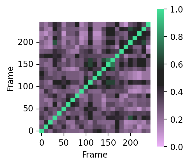
To compare binding modes in your trajectory, it’s possible to compute the entire similarity matrix:
import pandas as pd
import seaborn as sns
from matplotlib import pyplot as plt

# Tanimoto similarity matrix
bitvectors = fp.to_bitvectors()
similarity_matrix = []
for bv in bitvectors:
    similarity_matrix.append(DataStructs.BulkTanimotoSimilarity(bv, bitvectors))
similarity_matrix = pd.DataFrame(similarity_matrix, index=df.index, columns=df.index)

# display heatmap
fig, ax = plt.subplots(figsize=(3, 3), dpi=200)
colormap = sns.diverging_palette(
    300, 145, s=90, l=80, sep=30, center="dark", as_cmap=True
)
sns.heatmap(
    similarity_matrix,
    ax=ax,
    square=True,
    cmap=colormap,
    vmin=0,
    vmax=1,
    center=0.5,
    xticklabels=5,
    yticklabels=5,
)
ax.invert_yaxis()
plt.yticks(rotation="horizontal")
fig.patch.set_facecolor("white")
Visualisation#
There are a few different options builtin when it comes to visualisation.
You can start by plotting the interactions over time:
# %matplotlib ipympl

fp.plot_barcode()
<Axes: xlabel='Frame'>

Tip
If you uncomment %matplotlib ipympl at the top of the above cell, you should be able to see an interactive version of the plot.
You can also display the interactions in a 2D interactive diagram if you have a small peptide (not the case here so the plot below won’t be readable but that’s ok):
view = fp.plot_lignetwork(small_protein_mol)
view
This diagram is interactive, you can:
zoom and pan,
move residues around,
click on the legend to display or hide types of residues or interactions,
hover an interaction line to display the distance.
Note
After arranging the residues to your liking, you can save the plot as a PNG image with:
view.save_png()
Note that this only works in notebooks and cannot be used in regular Python scripts.
You can generate 2 types of diagram with this function, controlled by the kind argument:
frame: shows a single specific frame (specified withframe, corresponds to the frame number in the simulation).aggregate(default): the interactions from all frames are grouped and displayed. An optionalthresholdparameter controls the minimum frequency required for an interaction to be displayed (default0.3, meaning that interactions occuring in less than 30% of frames will be hidden). The width of interactions is linked to the frequency.
Tip
Make sure to check the Ligand-Protein tutorial for more examples on this plot.
You can also visualize this information in 3D.
Up to now we’ve only been using the default fingerprint generator, but you can optionally enable the count parameter to enumerate all occurences of an interaction (the default fingerprint generator will stop at the first occurence), and then ProLIF will automatically display the occurence with the smallest distance. You can show all of them with display_all=True.
fp_count = plf.Fingerprint(count=True)
fp_count.run(u.trajectory[0:1], small_protein_selection, large_protein_selection)
<prolif.fingerprint.Fingerprint: 9 interactions: ['Hydrophobic', 'HBDonor', 'HBAcceptor', 'PiStacking', 'Anionic', 'Cationic', 'CationPi', 'PiCation', 'VdWContact'] at 0x7b2ce1675710>
frame = 0
# seek specific frame
u.trajectory[frame]
small_protein_mol = plf.Molecule.from_mda(small_protein_selection)
large_protein_mol = plf.Molecule.from_mda(large_protein_selection)
# display
view = fp_count.plot_3d(
    small_protein_mol, large_protein_mol, frame=frame, display_all=False
)
view
3Dmol.js failed to load for some reason. Please check your browser console for error messages.
<prolif.plotting.complex3d.Complex3D at 0x7b2cea94ab90>
As in the lignetwork plot, you can hover atoms and interactions to display more information.
Once you’re satisfied with the orientation, you can export the view as a PNG image with:
view.save_png()
Note that this only works in notebooks and cannot be used in regular Python scripts.
Another powerfull visualization option for protein-protein interaction is to use networks to abstract away atomic details.
networkx is a great library for working with graphs in Python, but since the drawing options are quickly limited we will also use pyvis to create interactive plots. The following code snippet will convert each residue in our selections to a node, each interaction to an edge, and the occurence of each interaction between residues will be used to control the weight and thickness of each edge.
from html import escape
import networkx as nx
import pandas as pd
from IPython.display import HTML
from matplotlib import colormaps, colors
from pyvis.network import Network


def make_graph(
    values: pd.Series,
    df: pd.DataFrame,
    node_color=["#FFB2AC", "#ACD0FF"],
    node_shape="dot",
    edge_color="#a9a9a9",
    width_multiplier=1,
) -> nx.Graph:
    """Convert a pandas DataFrame to a NetworkX object

    Parameters
    ----------
    values : pandas.Series
        Series with 'ligand' and 'protein' levels, and a unique value for
        each lig-prot residue pair that will be used to set the width and weigth
        of each edge. For example:

            ligand  protein
            LIG1.G  ALA216.A    0.66
                    ALA343.B    0.10

    df : pandas.DataFrame
        DataFrame obtained from the fp.to_dataframe() method
        Used to label each edge with the type of interaction

    node_color : list
        Colors for the ligand and protein residues, respectively

    node_shape : str
        One of ellipse, circle, database, box, text or image, circularImage,
        diamond, dot, star, triangle, triangleDown, square, icon.

    edge_color : str
        Color of the edge between nodes

    width_multiplier : int or float
        Each edge's width is defined as `width_multiplier * value`
    """
    lig_res = values.index.get_level_values("ligand").unique().tolist()
    prot_res = values.index.get_level_values("protein").unique().tolist()

    G = nx.Graph()
    # add nodes
    # https://pyvis.readthedocs.io/en/latest/documentation.html#pyvis.network.Network.add_node
    for res in lig_res:
        G.add_node(
            res, title=res, shape=node_shape, color=node_color[0], dtype="ligand"
        )
    for res in prot_res:
        G.add_node(
            res, title=res, shape=node_shape, color=node_color[1], dtype="protein"
        )

    for resids, value in values.items():
        label = "{} - {}\n{}".format(
            *resids,
            "\n".join(
                [
                    f"{k}: {v}"
                    for k, v in (
                        df.xs(resids, level=["ligand", "protein"], axis=1)
                        .sum()
                        .to_dict()
                        .items()
                    )
                ]
            ),
        )
        # https://pyvis.readthedocs.io/en/latest/documentation.html#pyvis.network.Network.add_edge
        G.add_edge(
            *resids,
            title=label,
            color=edge_color,
            weight=value,
            width=value * width_multiplier,
        )

    return G
data = df.T.groupby(level=["ligand", "protein"], sort=False).sum().T.astype(bool).mean()

G = make_graph(data, df, width_multiplier=8)

# color each node based on its degree
max_nbr = len(max(G.adj.values(), key=lambda x: len(x)))
blues = colormaps.get_cmap("Blues")
reds = colormaps.get_cmap("Reds")
for n, d in G.nodes(data=True):
    n_neighbors = len(G.adj[n])
    # show the smaller domain in red and the larger one in blue
    palette = reds if d["dtype"] == "ligand" else blues
    d["color"] = colors.to_hex(palette(n_neighbors / max_nbr))

# convert to pyvis network
width, height = (700, 700)
net = Network(width=f"{width}px", height=f"{height}px", notebook=True, heading="")
net.from_nx(G)

html_doc = net.generate_html(notebook=True)
iframe = (
    f'<iframe width="{width+25}px" height="{height+25}px" frameborder="0" '
    'srcdoc="{html_doc}"></iframe>'
)
HTML(iframe.format(html_doc=escape(html_doc)))
Warning: When cdn_resources is 'local' jupyter notebook has issues displaying graphics on chrome/safari. Use cdn_resources='in_line' or cdn_resources='remote' if you have issues viewing graphics in a notebook.